B-Trees - Database storage internals

Some of the most popular databases out there (PostgreSQL, MySQL, MongoDB, etc) use b-trees for their indexes. In this article, we’re going to learn how they work and understand why they are used.

Files

Before we understand how databases store information, we need to understand how computers store information.

When we want to persist data, we use the file system API. This API allows us to open files for reading, writing or appending. When a file is opened, it’s loaded into memory. Once the data is in memory, we can access bytes sequentially or in any order we desire (Random Access).

Unsorted data

Suppose we want to store a key-value relationship. Let’s say our key is a 32-bit integer representing a unique identifier for a person. And the value is a string with the name of the person.

A logical representation of our data looks like this:

1
2
3
1 Carlos
2 Jose
3 Alberto

But it would be a little more accurate to show it like this (In hexadecimal):

1
2
3
00 00 00 01 43 61 72 6C 6F 73 0A
00 00 00 02 4A 6F 73 65 0A
00 00 00 03 41 6C 62 65 72 74 6F 0A

Notice how we use 4 bytes to represent our key, so 1, becomes 00 00 00 01. We use a byte (In real life we would probably use multiple bytes for UTF-8, but we are using ASCII for simplicity) for each character on the value, so Carlos becomes 43 61 72 6C 6F 73. We also add a 0A byte to denote the end of a record. In the example above, we put each record in a new line, but in a file each record comes immediately after the next one.

Inserting data is easy, we just add new records at the end of the file:

1
2
3
4
1 Carlos
2 Jose
3 Alberto
4 Maria

Or

1
2
3
4
00 00 00 01 43 61 72 6C 6F 73 0A
00 00 00 02 4A 6F 73 65 0A
00 00 00 03 41 6C 62 65 72 74 6F 0A
00 00 00 04 4D 61 72 69 61 0A

If we need to find the value corresponding to a key, we need to scan the whole file until we find the key. To get the value, we read the following bytes until we find 0A. If this file becomes large, this can be very time-consuming.

We could make things a little better if we put the keys in one file and the values in another file. Let’s dump our values into a new file:

1
2
3
4
43 61 72 6C 6F 73 0A
4A 6F 73 65 0A
41 6C 62 65 72 74 6F 0A
4D 61 72 69 61 0A

In our keys file, we can include a pointer to the offset where the value for that key starts:

1
2
3
4
00 00 00 01 00 00 00 00
00 00 00 02 00 00 00 07
00 00 00 03 00 00 00 0C
00 00 00 04 00 00 00 14

Since our keys file is now smaller, it will be faster to scan through the entire file.

Indexes

Splitting the keys and the values works like a kind of index, but not a very good one. Good indexes provide a way to perform fast searches that don’t require scanning all the data.

When it comes to fast search, we have a few well known tools at our disposal. One of them could be a binary search. The problem with a binary search is that it requires our index to be sorted, which could be expensive. Imagine we have this index:

1
2
3
4
11
12
13
14

And we want to insert key 5. We basically need to rewrite the whole file so it looks like this:

1
2
3
4
5
5
11
12
13
14

Rewriting the full index for every insert would make our database incredibly slow very quickly.

Another data structure that allows for very fast search, is a hash table, but it comes with a similar issue. When we run out of space in the underlying storage, we need to allocate more space and move all the data to the new location.

This is where B-Trees become important. But before we look into them, let’s look at a more well known tree.

Binary Search Trees (BST)

If you have studied data structures, you are probably familiar with BSTs. A BST is defined as a tree where the value of a node is greater than all the nodes on its left subtree and lower than all nodes on its right subtree.

Simple BSTs are easy to implement. If we start with an empty tree, and we add a value, we just put it in the root:

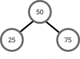
If we want to add another value, we compare it with the root. If it’s greater, we put it on the right, if it’s lower, we put it on the left:

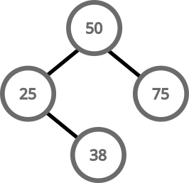
For inserting more values, we can do this recursively. We keep going left or right deep into the three until we find a spot to put our value:

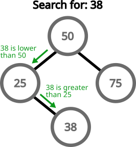
Searching for a value follows more or less the same pattern. Start at the root and go left or right accordingly:

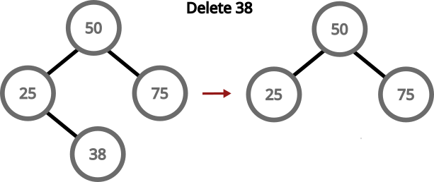
Deleting a node is a little more complicated in some scenarios. If we need to delete a leaf node, then it’s all smooth:

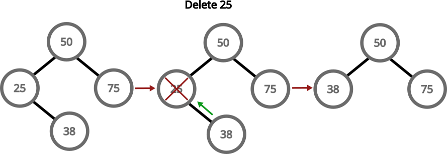
If we need to delete a node with only one child, then the child replaces the parent:

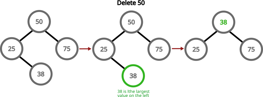
If we need to delete a node with two children, we can grab the largest number in the left subtree, replace the value of the node with the value of that node and then delete that largest number:

An update is just a delete, followed by an insert.

Balancing trees

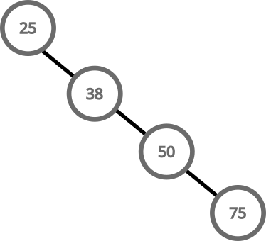
BSTs are supposed to make search operations fast, but if the tree is not balanced, we could end up with a tree like this:

Searching this tree has a complexity on O(n), because it performs a scan of all the elements in the tree to find a value.

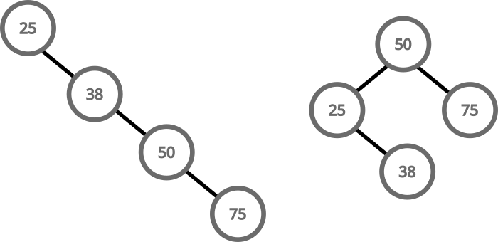
To keep searching a BST tree efficient, we need to keep the tree balanced. These two trees are equivalent, but one has a search complexity of O(n) and the other one of O(long(n)):

There are techniques that allow us to keep a BST balanced even as we insert and delete values. The most notable example being AVL trees. I have covered AVL trees in another article, so I’m not going to go over them here.

B-Trees

B-Trees are a more generalized version of a binary tree. Instead of a node having only 2 children, it can have M children. Having more children is beneficial for storage systems that allow writing and reading data in large chunks (such as file systems).

B-Trees must have the following characteristics:

• Every node has at most M children
• Every node, except for the root and the leaves, has at least M/2 children
• The root node has at least 2 children, unless it is a leaf
• All leaves appear on the same level
• A non-leaf node with k children contains k−1 keys

The degree of a B-Tree (M) is often chosen based on the block size of the storage device.

Imagine our system has the following characteristics:

• Block size is 4 KB (4096 Bytes)
• Payload is 64 bits (8 Bytes)
• Pointers are 64 bits (8 Bytes)

We can calculate M with this equation:

1
8(M) + 8(M - 1) = 4096

If we solve for M:

1
2
3
4
8M + 8M - 8 = 4096
16M = 4096 + 8
16M = 4104
M = 256.5

B-Trees with degrees in the hundreds are typical for real world databases, but we’ll start with a lower number to make them easier to understand.

Let’s look at how a B-Tree with a degree of 3 works. We start by inserting 50 to the tree:

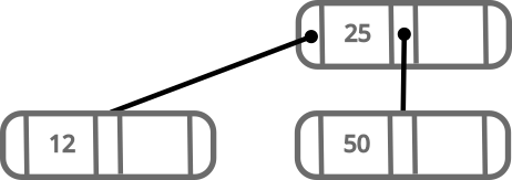
The next number we insert is going to be added in the correct order in the same node. Let’s insert 25:

Since 25 is lower than 50, it’s inserted on the left.

Since our B-Tree has a degree of 3, it can have at most 2 values per node. This means, next time we insert a value, we’ll need to rebalance the tree.

Let’s say we want to insert 12. We follow these steps:

• Get the root node
• Because:
  • 12 is lower than 25
  • The node has no left child
  • The node is full
• Order the 3 numbers: 12, 25, 50
• Grab 12 and move it to a new node on the left
• Grab 50 and move it to a new node on the right
• Make 25 the new root with the other two nodes as children

We again have a nicely balanced tree; this time with more than one node.

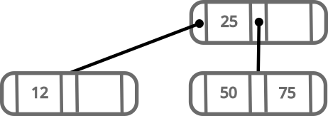
Let’s now see what happens when we add 75:

New values are always added at leaf nodes and only move up when balancing happens.

If we try to add 87, we’ll run into our right node having more than 2 values. In this case, we follow a similar process than the one we did before.

• Order the 3 numbers: 50, 75, 87
• Grab 87 and move it to a new node on the right
• Move 75 to the root node
• Make the middle child of the root, point to 50 and the right child, point to 87

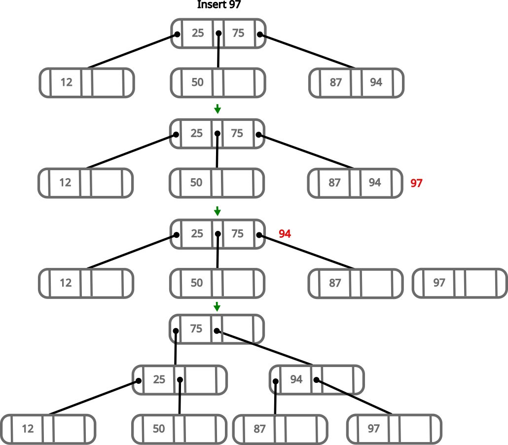
The insertion algorithm for B-trees is recursive, so we follow the same procedure when parent nodes get full. We can easily insert 94 in the right leaf of our tree, but let’s see what happens when we try to insert 97.

• Order the 3 numbers in the right most subtree: 87, 94, 97
• Grab 97 and move it to a new node on the right
• Keep 87 on that node on the left side
• We try to move 94 to the parent, but since it’s full, we continue recursively
• We have values: 25, 75, 94
• We put 94 in a new node on the right
• We move 75 up and make it point to the left to 25 and to the right to 94

At this point, we can see that there are a lot of holes available in our nodes. This is good because it means, in many scenarios, we’ll be able to insert new values without having to rebalance the tree.

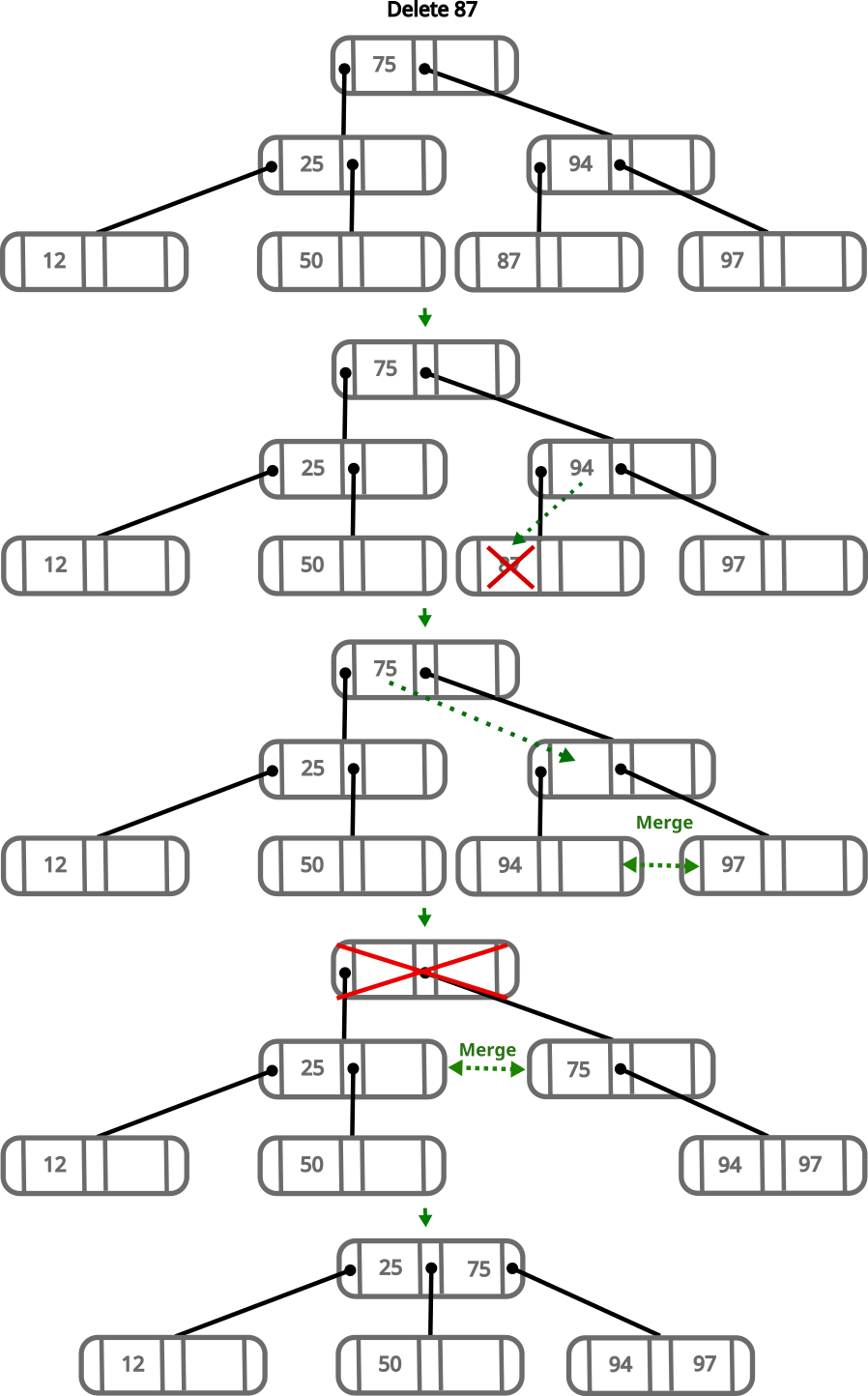
When deleting values, we have to consider that every node that is not a leaf or the root has to have at least M/2 children. For our tree, this means a node has to have at least 2 children. Let’s see what happens if we decide to delete 87.

• Deleting 87 leaves its parent with a single child
• To fix this, we move 94 to the node where 87 was
• This leaves the node where 94 was empty
• To fix this we move the parent down, but since it’s the root, we move it to the left child, and it becomes the new root

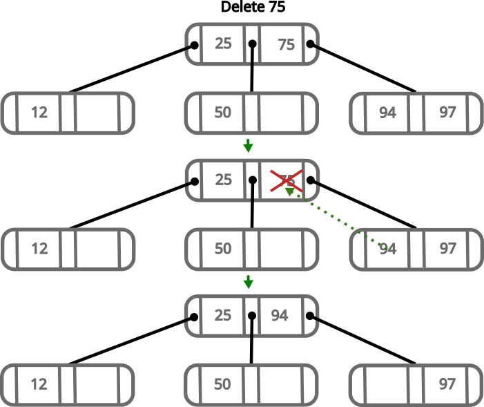
If we want to delete an intermediate value, for example 75, we need to follow the following steps:

• Remove 75
• Move 94 to where 75 was

As you can see, the algorithm is not very complicated, and it scales with the height of the tree. With high values of M the height of the tree increases slowly, thus making the algorithm very fast.

Conclusion

B-Trees are a very interesting data structure. They are very easy to manage in relation to how powerful they are.

The correct implementation of B-Trees on production databases is a little more complicated than explained here, as we need to deal with metadata and the file system, but the algorithm remains the same.