Have you ever had to draw an architecture diagram and found the repetitive clicking and dragging tedious? Did you have to do modifications to that diagram and found it complicated?
Graphviz is an open source graph visualization software that allows us to decribe a diagram using code, and have it automatically drawn for us. If the diagram needs to be modified in the future, we just need to modify the description and the nodes and edges will be repositioned automatically for us.
Drawing graphs
Before we start writing graphs, we need to learn how we can convert our code into an image so we can test what we are doing.
Webgraphviz.com can be used to draw graphs from a browser.
We can also install the command line tool in Ubuntu using apt:
1
sudo apt install graphviz
This will install, among other things, the dot CLI, which can be used to generate images from text files:
1
dot -Tpng input.gv -o output.png
In the example above we are specifying png as the output (-Tpng), but there are many options available. As we can see, the input files commonly use the gv extension.
DOT
DOT is the most common format used to describe graphs to be parsed by Graphviz.
Basics
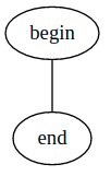
A simple graph has this form:
1
2
3
graph MyGraph {
  begin -- end
}
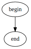
If we want to use a directed graph (one with arrows), we need to use digraph instead:
1
2
3
digraph MyGraph {
  begin -> end
}
Arrows can be in one direction or bidirectional:
1
2
3
4
digraph MyGraph {
  a -> b
  a -> c [dir=both]
}
![]()
Shapes
If we don’t like ovals, we can use other shapes:
1
2
3
4
5
6
7
8
9
10
11
12
13
14
15
16
17
18
19
digraph MyGraph {
  a [shape=box]
  b [shape=polygon,sides=6]
  c [shape=triangle]
  d [shape=invtriangle]
  e [shape=polygon,sides=4,skew=.5]
  f [shape=polygon,sides=4,distortion=.5]
  g [shape=diamond]
  h [shape=Mdiamond]
  i [shape=Msquare]
  a -> b
  a -> c
  a -> d
  a -> e
  a -> f
  a -> g
  a -> h
  a -> i
}
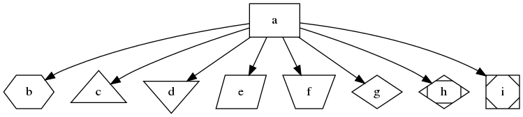
The different supported shapes can be found in the node shapes section of their documentation.
We can also add some color and style to our nodes:
1
2
3
4
5
6
7
8
9
10
11
12
13
14
15
16
17
18
19
20
21
22
23
digraph MyGraph {
  a [style=filled,color=green]
  b [peripheries=4,color=blue]
  c [fontcolor=crimson]
  d [style=filled,fillcolor=dodgerblue,color=coral4,penwidth=3]
  e [style=dotted]
  f [style=dashed]
  g [style=diagonals]
  h [style=filled,color="#333399"]
  i [style=filled,color="#ff000055"]
  j [shape=box,style=striped,fillcolor="red:green:blue"]
  k [style=wedged,fillcolor="green:white:red"]
  a -> b
  a -> c
  a -> d
  a -> e
  b -> f
  b -> g
  b -> h
  b -> i
  d -> j
  j -> k
}
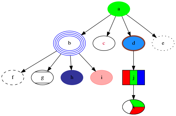
The different color names can be found in the color names documentation.
Arrows
Arrows’ tails and heads can also be modified:
1
2
3
4
5
6
7
8
digraph MyGraph {
  a -> b [dir=both,arrowhead=open,arrowtail=inv]
  a -> c [dir=both,arrowhead=dot,arrowtail=invdot]
  a -> d [dir=both,arrowhead=odot,arrowtail=invodot]
  a -> e [dir=both,arrowhead=tee,arrowtail=empty]
  a -> f [dir=both,arrowhead=halfopen,arrowtail=crow]
  a -> g [dir=both,arrowhead=diamond,arrowtail=box]
}
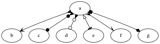
The different arrow types can be found in the arrow shapes documentation.
As well as adding styles to the arrow line:
1
2
3
4
5
6
7
8
9
10
11
digraph MyGraph {
  a -> b [color="black:red:blue"]
  a -> c [color="black:red;0.5:blue"]
  a -> d [dir=none,color="green:red:blue"]
  a -> e [dir=none,color="green:red;.3:blue"]
  a -> f [dir=none,color="orange"]
  d -> g [arrowsize=2.5]
  d -> h [style=dashed]
  d -> i [style=dotted]
  d -> j [penwidth=5]
}
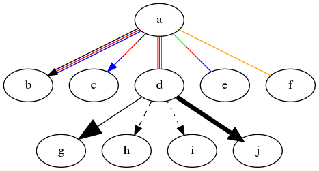
If we pay attention to the code and diagram above, we can see that when we specify multiple colors for an arrow, there will be one line for each color, if we don’t specify any weight. If we want a single arrow with multiple colors, at least one color has to specify the weight percentage of the line to cover:
1
  a -> e [dir=none,color="green:red;.3:blue"]
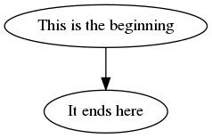
Labels
We can add labels to nodes:
1
2
3
4
5
digraph MyGraph {
  begin [label="This is the beginning"]
  end [label="It ends here"]
  begin -> end
}
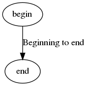
As well as vertices:
1
2
3
4
5
digraph MyGraph {
  begin
  end
  begin -> end [label="Beginning to end"]
}
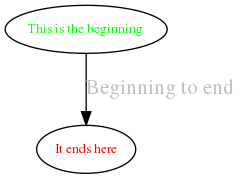
We can style our labels:
1
2
3
4
5
digraph MyGraph {
  begin [label="This is the beginning",fontcolor=green,fontsize=10]
  end [label="It ends here",fontcolor=red,fontsize=10]
  begin -> end [label="Beginning to end",fontcolor=gray,fontsize=16]
}
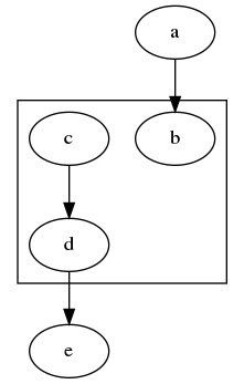
Clusters
Clusters are also called subgraphs. The name of a cluster needs to be start with cluster_, or it won’t be contained in a box.
1
2
3
4
5
6
7
8
digraph MyGraph {
  subgraph cluster_a {
    b
    c -> d
  }
  a -> b
  d -> e
}
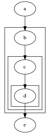
Clusters can be nested as neccessary:
1
2
3
4
5
6
7
8
9
10
11
12
13
digraph MyGraph {
  subgraph cluster_a {
    subgraph cluster_b {
      subgraph cluster_c {
        d
      }
      c -> d
    }
    b -> c
  }
  a -> b
  d -> e
}
HTML
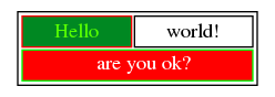
HTML allows us to create more complicated nodes that can be split into sections. Each section can be referred to in the graph independently:
1
2
3
4
5
6
7
8
9
10
11
12
13
14
15
16
17
18
19
20
21
22
23
24
25
26
27
28
29
30
31
digraph MyGraph {
    a [shape=plaintext,label=<
      <table>
        <tr>
          <td>Hello</td>
          <td>world!</td>
        </tr>
        <tr>
          <td colspan="2" port="a1">are you ok?</td>
        </tr>
      </table>
    >]
    b [shape=plaintext,label=<
      <table border="0" cellborder="1" cellspacing="0">
        <tr>
          <td rowspan="3">left</td>
          <td>top</td>
          <td rowspan="3" port="b2">right</td>
        </tr>
        <tr>
          <td port="b1">center</td>
        </tr>
        <tr>
          <td>bottom</td>
        </tr>
      </table>
    >]

    a:a1 -> b:b1
    a:a1 -> b:b2
}
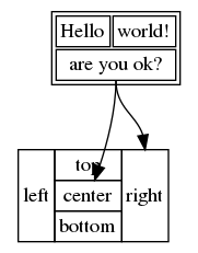
Only a subset of HTML can be used to create nodes, and the rules are pretty strict. In order for the node to display correctly, we need to set the shape to plaintext.
Another important thing to notice is the port attribute, which allows us to reference that specific cell by using a colon (a:a1).
We can style our HTML nodes, but we can only use a subset of HTML:
1
2
3
4
5
6
7
8
9
10
11
12
13
14
15
digraph MyGraph {
    a [shape=plaintext,label=<
      <table>
        <tr>
          <td color="#ff0000" bgcolor="#008822"><font color="#55ff00">Hello</font></td>
          <td>world!</td>
        </tr>
        <tr>
          <td colspan="2" color="#00ff00" bgcolor="#ff0000">
            <font color="#ffffff">are you ok?</font>
          </td>
        </tr>
      </table>
    >]
}
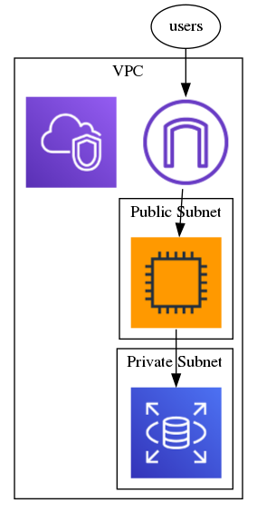
Images
Sometimes we want to use specify icons for our nodes, this can be done with the image attribute:
1
2
3
4
5
6
7
8
9
10
11
12
13
14
15
16
17
18
19
20
21
22
23
24
25
digraph MyGraph {
  ec2 [shape=none,label="",image="icons/ec2.png"]
  igw [shape=none,label="",image="icons/igw.png"]
  rds [shape=none,label="",image="icons/rds.png"]
  vpc [shape=none,label="",image="icons/vpc.png"]

  subgraph cluster_vpc {
    label="VPC"

    subgraph cluster_public_subnet {
      label="Public Subnet"
      ec2
    }

    subgraph cluster_private_subnet {
      label="Private Subnet"
      ec2 -> rds
    }

    vpc
    igw -> ec2
  }

  users -> igw
}
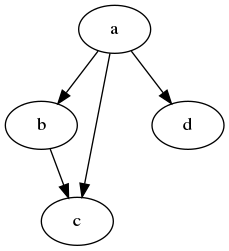
Ranks
Ranks are one of the most complicated things to understand, since they alter how the rendering engine works. Here I’m just going to cover some of the basic things that I find useful.
A Graph will normally be rendered top to bottom:
1
2
3
4
5
6
digraph MyGraph {
  a -> b
  b -> c
  a -> d
  a -> c
}
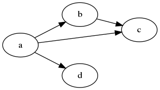
Using the rankdir attribute, we can render it left to right:
1
2
3
4
5
6
7
8
digraph MyGraph {
  rankdir=LR

  a -> b
  b -> c
  a -> d
  a -> c
}
Ranking can also be used to force a node to be at the same level as another node:
1
2
3
4
5
6
7
8
9
10
digraph MyGraph {
  rankdir=LR

  a -> b
  b -> c
  a -> d
  a -> c

  {rank=same;c;b}
}
![]()
In the example above we use rank=same to align node c with node b.
The rankdir attribute is global, so it can’t be changed inside a cluster, but using rank we can simulate an LR direction inside clusters:
1
2
3
4
5
6
7
8
9
10
11
12
13
14
15
16
17
18
digraph MyGraph {
  subgraph cluster_A {
    a1 -> a2
    a2 -> a3

    {rank=same;a1;a2;a3}
  }

  subgraph cluster_B {
    a3 -> b1
    b1 -> b2
    b2 -> b3

    {rank=same;b1;b2;b3}
  }

  begin -> a1
}
![]()
We can combine rank with constraint=false to create more compact graphs:
1
2
3
4
5
6
7
8
9
10
11
12
13
14
15
16
17
18
19
20
21
22
23
digraph MyGraph {
  subgraph cluster_A {
    a1
    a2
    a3
    {rank=same;a1;a2;a3}
  }

  subgraph cluster_B {
    b1
    b2
    b3

    {rank=same;b1;b2;b3}
  }

  begin -> a1
  a1 -> a2 [constraint=false]
  a2 -> a3 [constraint=false]
  a3 -> b1
  b1 -> b2
  b2 -> b3
}

Rank can also be used to specify the distance between each node:
1
2
3
4
5
6
7
digraph MyGraph {
  rankdir=LR
  ranksep=1
  a -> b
  b -> c
  c -> d
}
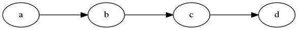
The default value for ranksep is .5.
Conclusion
In this post we learned how we can use Graphviz to generate graphs based on a declarative language. This has made it a lot easier for me to draw architecture diagrams and modify them in the future.
I presented the features that I consider most important for everyday use, but there are a good amount of features that I didn’t cover and frankly, I don’t understand.
productivity